Inertial Confinement Fusion

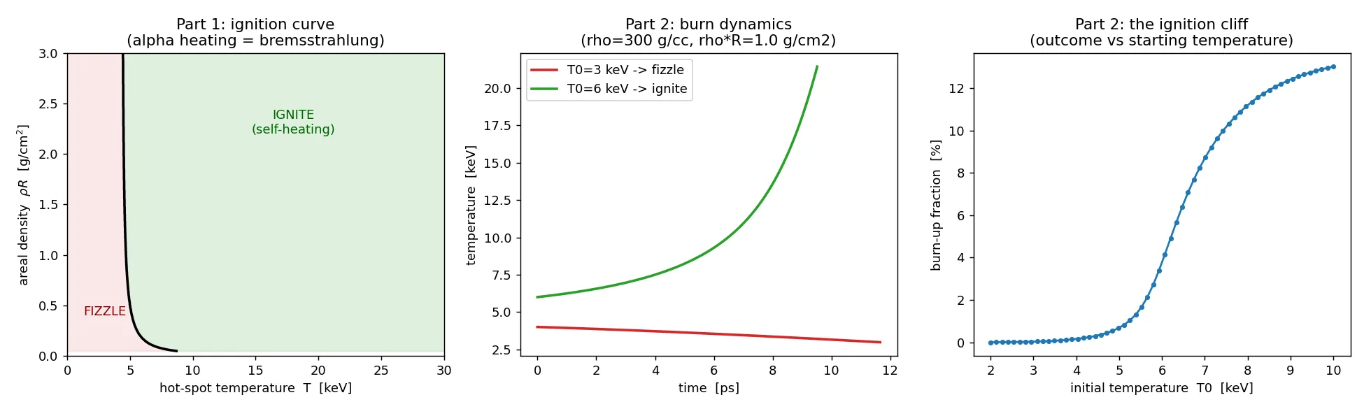
A zero-dimensional model of the ignition physics that decides whether a DT hot spot ignites, using the Bosch–Hale fusion reactivity fit (accurate 0.2–100 keV) so the numbers are quantitative, not hand-waved. It balances three effects: alpha self-heating (3.5 MeV alphas redepositing their energy, a positive feedback), bremsstrahlung radiation loss (∝ n² √T), and alpha confinement — alphas only stop locally once the areal density ρR clears their ~0.3 g/cm² range. The figure shows three things: the ignition curve in the (T, ρR) plane, the boundary where alpha heating overtakes radiation, below which you cannot ignite at any density; the burn dynamics, where at the same ρR a 4 keV start decays (fizzle) while a 6 keV start runs away to 21 keV (ignite), the same physics just 2 keV apart; and the ignition cliff, where burn-up versus starting temperature is flat and negligible, then rockets up over a ~1 keV window. The headline result falls straight out of the alpha-versus-bremsstrahlung balance: an ideal ignition temperature of 4.35 keV, the textbook value, not a hardcoded input. This burn-up function becomes the yield metric every later stage is scored against.

0-D hot-spot ignition: alpha self-heating versus bremsstrahlung sets an ignition boundary near 4.35 keV and ρR ≈ 0.3 g/cm². The right panel is the "ignition cliff" — burn-up jumps orders of magnitude over a ~1 keV window.

↳ feeds the ignition cliff → the yield model

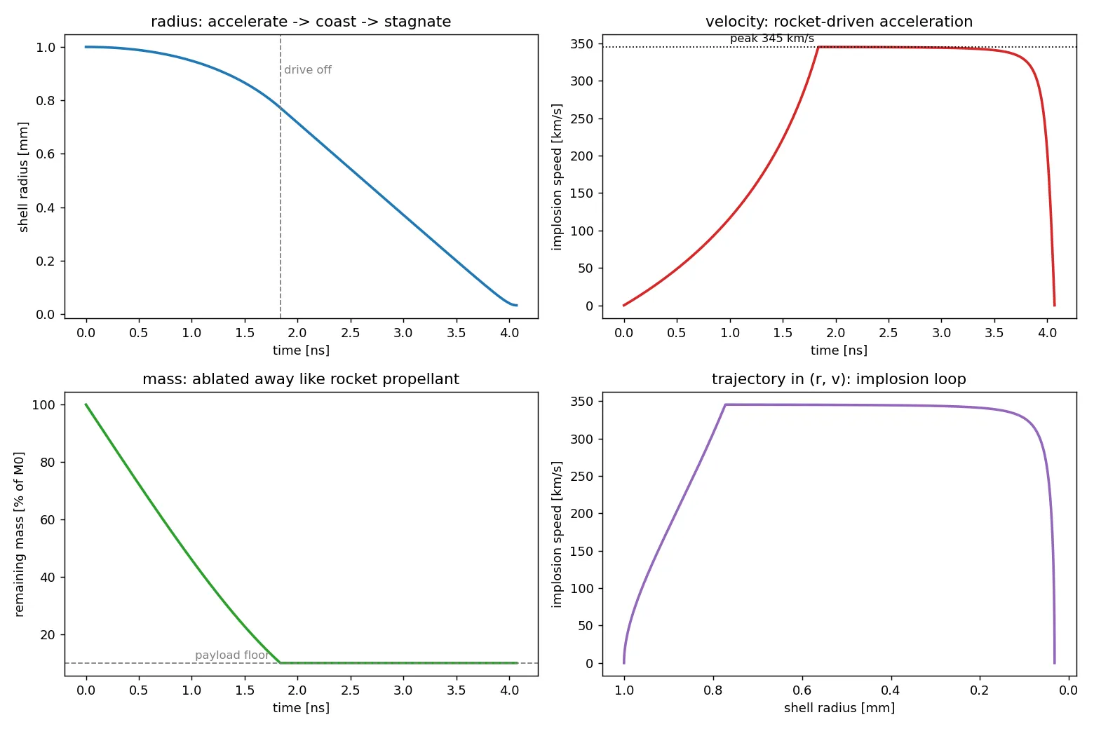
A lumped rocket model of the implosion: the ablator blows off and, by reaction, drives the shell inward to a huge velocity, and a central adiabatic gas cushion decelerates it at stagnation. The four panels show the three phases — rocket-driven acceleration, coast, and stagnation on the central gas. For a NIF-scale toy target it ignites: implosion velocity 345 km/s (the rocket equation v = v_ex · ln(M₀/M_payload) predicts 345.4, a cross-check that matches to 0.1 km/s), 90 percent of the mass ablated leaving a 10 percent payload, 17.9 kJ of kinetic energy, a convergence ratio of 31, a stagnation ρR of 2.27 g/cm² (clearing the 0.3 g/cm² bar), and a hot-spot temperature of 5.15 keV (clearing the 4.3 keV bar). Those stagnation conditions feed straight into the 0-D ignition bar. The biggest simplification, documented in the code, is that there is no Rayleigh–Taylor instability yet — the effect that most limits real implosions, which the next stages add.

The capsule as a rocket: the ablator blows off and drives the shell inward to a peak 345 km/s (matching the rocket equation), leaving a ~10% payload that stagnates and ignites.

↳ feeds g and v_imp → RT mechanics, convergent RT

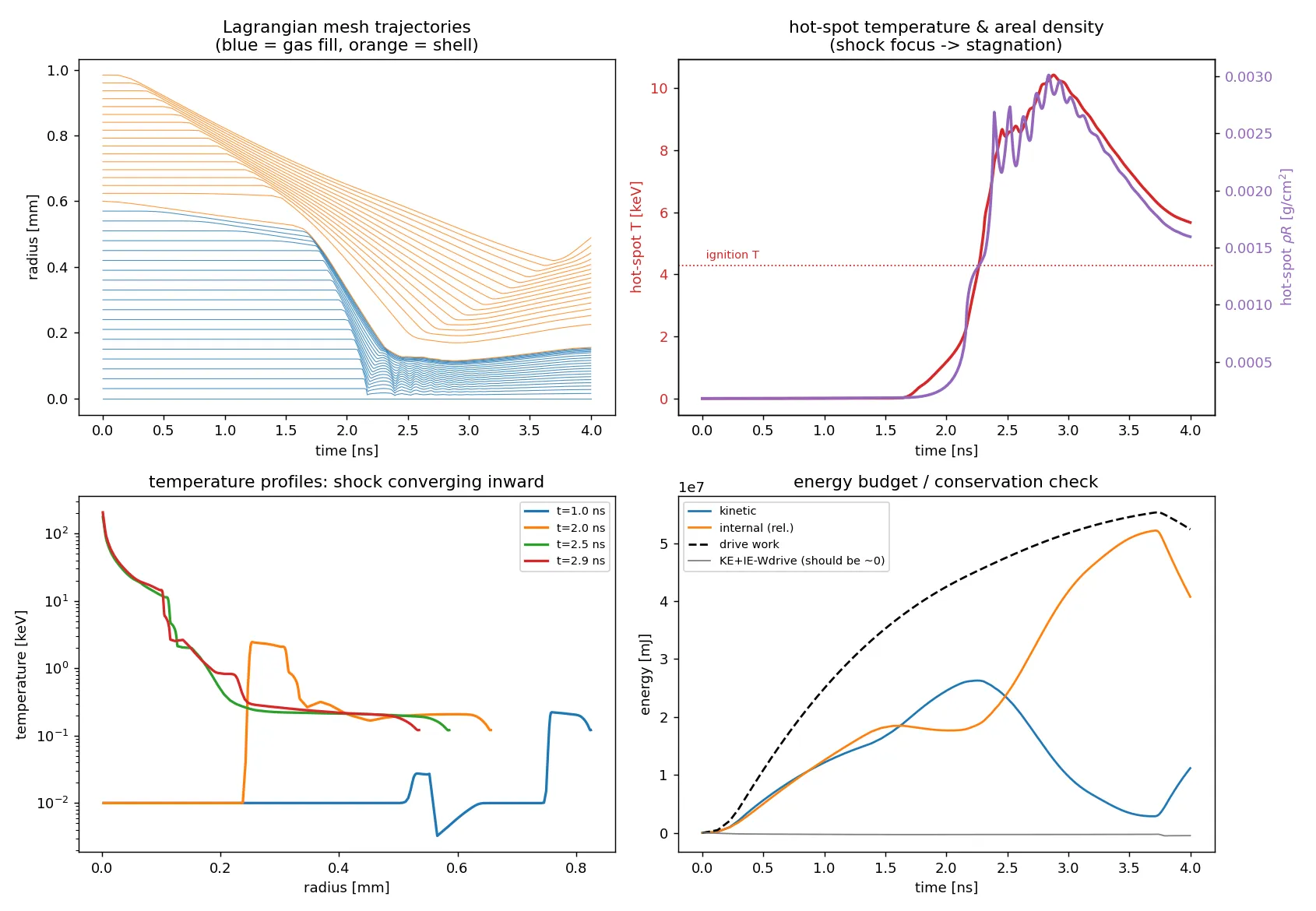
Where the 0-D and rocket models estimate the stagnation state, this spherical 1-D Lagrangian hydro solve computes it from the PDEs. It uses the classic staggered-grid scheme (von Neumann–Richtmyer, Wilkins): fixed Lagrangian mass zones, nodes carrying radius and velocity, artificial viscosity for shock capture, an ideal-gas EOS (γ = 5/3), a reflecting center and a pressure-driven outer boundary, over ~220 zones. A dense DT shell is driven inward, acts as a piston on the central gas fill, and launches a shock that converges on the origin to form the hot spot before rebounding — you can watch the shell trajectories pinch at r = 0 in the mesh plot. At a 150 Mbar drive it reaches stagnation at 2.9 ns, a mass-averaged hot-spot temperature of 10.4 keV, and conserves energy to −0.9 percent (the artificial-viscosity leak, the honest error bar on the peak temperature). Read honestly, the hot spot gets hot (clearing the 4.3 keV ignition temperature) but not dense (ρR much less than 0.3 g/cm²) — the correct signature of a lossless single-shock toy that only converges about 9×; building areal density is exactly what ablative compression buys you. The second figure is the verification suite: the same scheme run against three problems with exact solutions — the Sod shock tube (L1 density error 0.0015 versus the exact Riemann solution), the spherical Noh converging shock (post-shock plateau ρ = 61 versus exact 64, which shows the famous Noh wall-heating artifact every Lagrangian code has), and the Sedov blast (radius growing as t^0.398 versus exact 0.4, compression 5.6 versus exact 6). Passing these means the ICF results, and any ML trained on the solver, rest on a verified scheme, not a plausible-looking one.

A resolved 1-D spherical Lagrangian hydro solve — a driven shell launches a shock that converges to a ~10 keV hot spot, conserving energy to ≈1%.Verification of the 1-D Lagrangian scheme against three problems with exact solutions: the Sod shock tube (L1 density error 0.0015 vs the exact Riemann solution), the spherical Noh converging shock (post-shock plateau ρ = 61 vs exact 64, showing the classic Noh wall-heating artifact), and the Sedov blast (R ∝ t^0.398 vs exact 0.4, compression 5.6 vs exact 6). Passing these means the ICF results rest on a verified scheme.

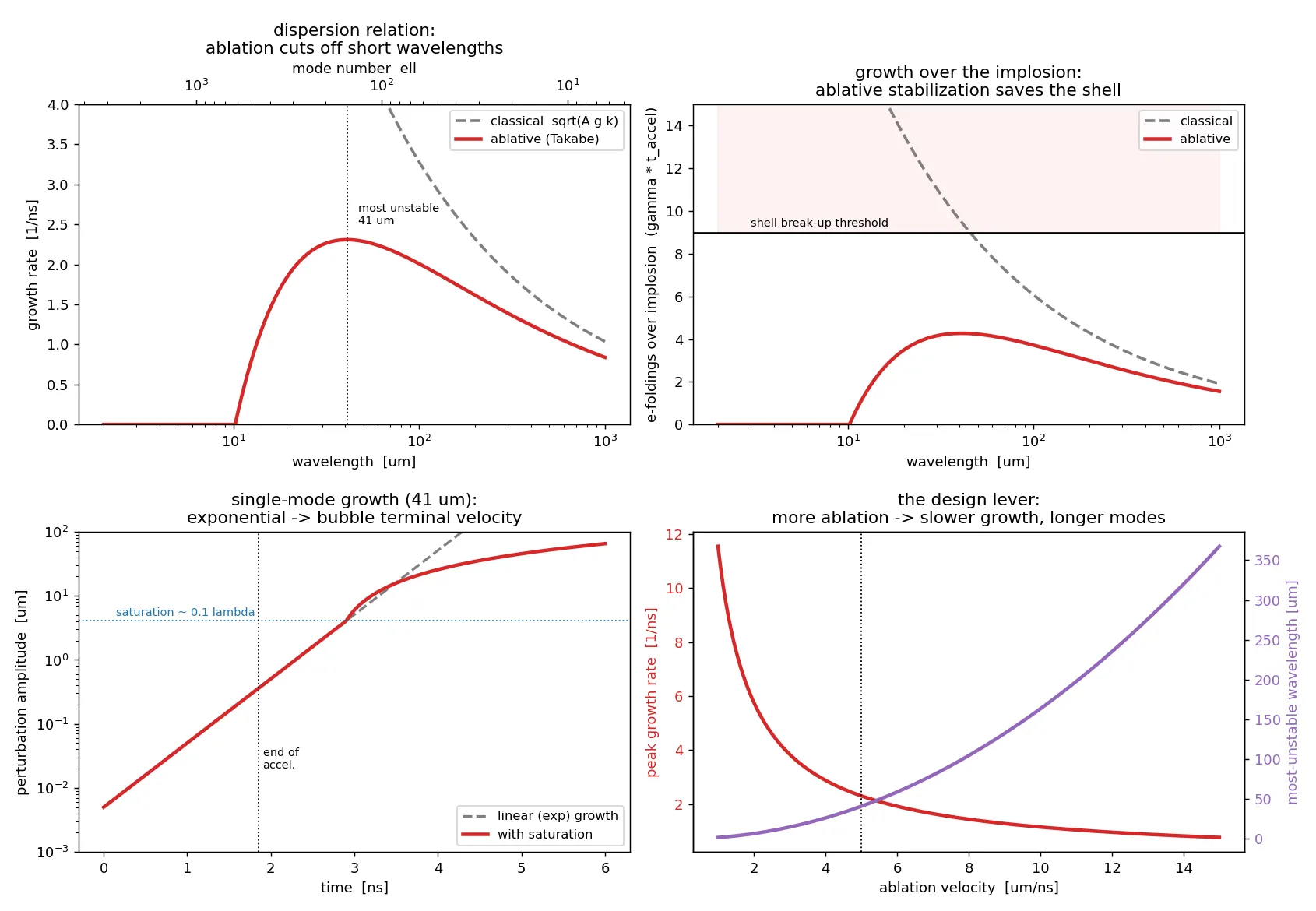
The linear and weakly-nonlinear theory of ablation-front Rayleigh–Taylor instability — the design constraints, in four panels. It contrasts the classical dispersion relation γ = √(A g k), which grows without bound at short wavelength, with the ablative (Takabe) form γ = α√(A g k) − β k V_ablation, which cuts off short wavelengths and selects a single most-dangerous mode near 41 µm (spherical-harmonic mode ℓ ≈ 150). The punchline is the growth over the implosion: across the ~1.85 ns acceleration a 5 nm surface ripple grows ×72 under ablative RT, to 0.36 µm, safely under the 40 µm shell — while without ablative stabilization the same ripple would grow ×13000 and break the shell up. Ablation is what holds ICF capsules together. The nonlinear panel shows the mode saturating near 0.1λ and then rising at the bubble terminal velocity, and the design-lever panel shows the peak growth rate scaling as 1/V_ablation, so faster ablation buys a smoother, longer-wavelength implosion at the cost of burning away more shell — the rocket-model trade.

Rayleigh–Taylor mechanics at the ablation front: the classical vs ablative (Takabe) dispersion relation that cuts off short wavelengths, the e-foldings over the implosion (ablative stabilization holds a 5 nm ripple to sub-micron — ×72 vs ×13000 without it), nonlinear bubble saturation, and the design lever, growth rate ∝ 1/ablation velocity.

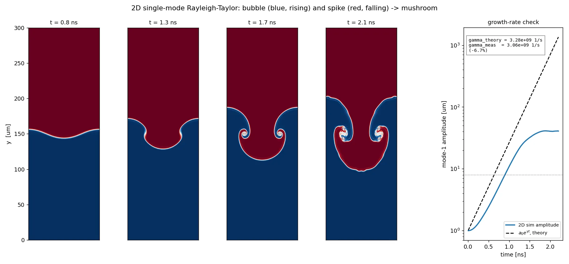
A real 2-D simulation that drops the linear assumption and grows the instability directly: an incompressible Boussinesq flow (vorticity–streamfunction with an FFT Poisson solve and semi-Lagrangian advection), heavy fluid on light, a single-mode ripple, gravity. The ripple grows into the classic light rising bubble and heavy falling spike, and the spike flanks roll up into the mushroom cap via Kelvin–Helmholtz — the picture everyone recognizes. Then the validation: it measures the early-time growth rate off the flow and compares to linear theory, √(A g k) = 3.28×10⁹ per second versus a measured 3.06×10⁹, an agreement of −6.7 percent. The residual is honest and visible in the growth-rate panel — the amplitude starts below the exponential because the flow begins at rest (cosh, not exp), and the starting interface has finite thickness, both of which slightly suppress the measured rate. Matching √(A g k) ties this simulation back to the dispersion relation the mechanics stage is built on.

2-D single-mode Rayleigh–Taylor instability growing from ripple to mushroom, with the measured growth rate matching linear theory to within ~7% — the instability that threatens implosion symmetry.

↳ feeds validates the RT growth rate

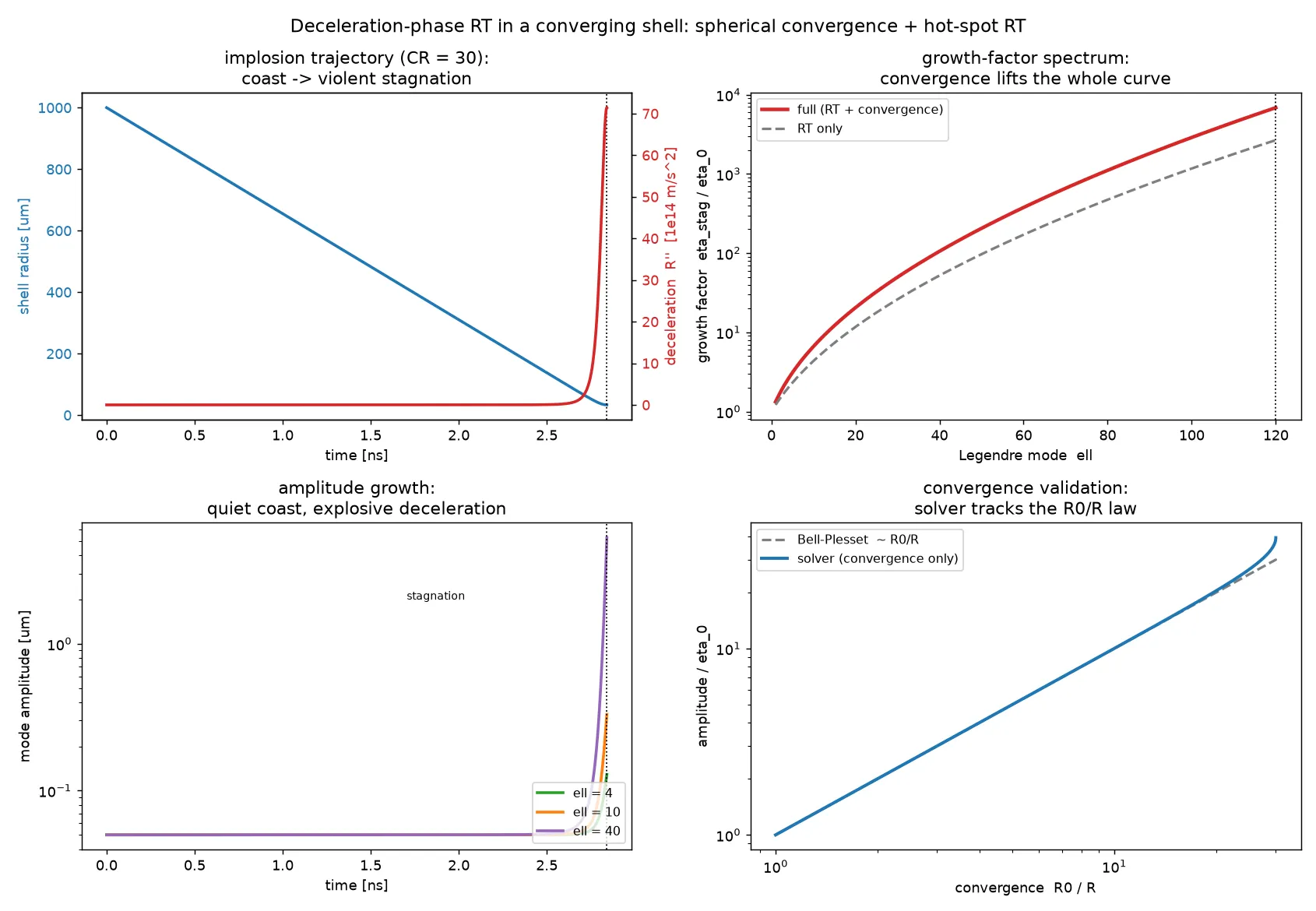
Extends Rayleigh–Taylor to the two effects a planar code cannot show, both of which make ICF spherical. First, deceleration-phase RT: at stagnation the light hot spot decelerates the heavy dense shell, and the effective gravity (the deceleration) peaks at about 37× the acceleration-phase g. There is no mass ablation at this interface, so no Takabe stabilization saves it — this is the RT that mixes cold fuel into the hot spot and quenches ignition, the second and more ignition-relevant place RT bites. Second, Bell–Plesset spherical convergence: in a converging implosion a mode amplitude grows geometrically as roughly R₀/R even without RT, and the local wavenumber sweeps upward as the shell shrinks. It integrates an implosion trajectory (coast into an adiabatic-gas stagnation, auto-tuned to convergence ratio 30) and grows each Legendre mode along it with a linearized interface ODE carrying both the convergence and the RT terms. It is anchored in both limits: the planar limit recovers the growth rate √(A g k) to −0.0 percent, and the convergence-only limit recovers the Bell–Plesset R₀/R law. It produces the growth-factor spectrum the drive-asymmetry stage amplifies.

Deceleration-phase Rayleigh–Taylor in a converging shell: the implosion trajectory and violent stagnation (peak deceleration ~37× the acceleration-phase g), the growth-factor spectrum that spherical convergence lifts, and validation that the solver recovers the Bell–Plesset R₀/R law.

↳ feeds growth factors → drive asymmetry

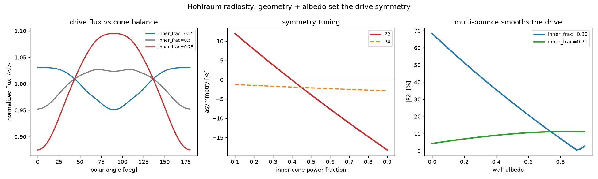
A multi-bounce radiosity calculation of where the X-ray drive symmetry comes from — the radiation bath a gold hohlraum delivers to the capsule. The wall re-emits a fraction of every X-ray that lands on it — the albedo, about 0.85 — so the radiation bounces many times before it escapes the laser-entrance hole or is absorbed by the capsule, and that bouncing is what smooths the drive. The transport is solved as a linear radiosity system over axisymmetric rings, P = E + albedo · VFᵀ · P, then the equilibrium wall brightness is integrated onto the capsule and decomposed into Legendre modes. It is validated by construction: the odd modes vanish to about 1e-16 (top-bottom symmetry); raising the albedo smooths the drive, dropping the P2 asymmetry at a fixed cone imbalance from about 68 percent at single bounce to a few percent by albedo ≈ 0.9; the inner-versus-outer laser-cone balance tunes P2 through zero (symmetric near an inner-cone fraction of 0.40); and a bigger entrance hole makes colder poles and drops P2. Its geometry-to-modes map is the input the next two stages consume.

A multi-bounce radiosity model of hohlraum drive symmetry — the X-ray bath the gold wall delivers to the capsule after many reflections — showing how the wall albedo smooths the drive and how the laser-cone balance tunes the P2 asymmetry through zero.

↳ feeds a2, a4 → drive asymmetry

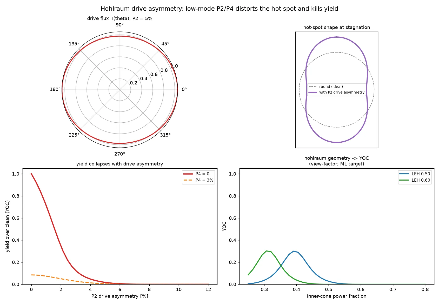
Couples low-mode P2 and P4 drive asymmetry to lost yield — the coupling that turns a geometry knob into a number the optimizer can chase. The drive asymmetry becomes a velocity asymmetry, then a ballistic offset, amplified by the convergent-RT growth factors, that distorts the hot spot into a peanut. That distortion feeds the same 0-D ignition model: residual kinetic energy lowers the hot-spot temperature and the thin peanut waist lowers the confining areal density, and the yield is the burn-up of that degraded hot spot relative to a round one. The sharp yield-over-clean collapse is the ignition cliff, not a fitted curve — 1 percent P2 gives YOC 0.72, 2 percent gives 0.35, 5 percent gives 0.02. A percent or two is enough to fall off the cliff, which is exactly why NIF holds drive symmetry to sub-percent.

Low-mode drive asymmetry distorts the hot spot into a peanut; fed into the 0-D ignition model, the yield collapse falls straight out of the ignition cliff — a percent or two of P2 is enough, which is why NIF holds drive symmetry to sub-percent.

↳ feeds YOC → ML

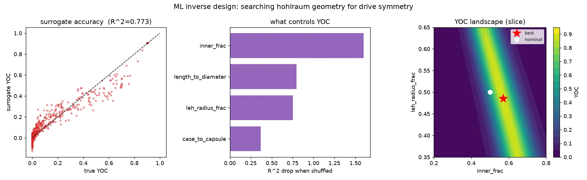
The full chain — hohlraum geometry to view-factor symmetry to hot-spot shape to yield-over-clean — is a cheap, deterministic forward model, so the ML does not replace the physics; it learns the forward model and then searches it. A scikit-learn MLPRegressor surrogate trained on Latin-hypercube samples, plus a differential-evolution active-learning loop, searches the 4-D geometry space (case-to-capsule ratio, length-to-diameter, entrance-hole size, and cone balance). The active-learning loop proposes the surrogate optimum, verifies it against the real forward model, and folds it back in, so the surrogate sharpens exactly where the optimum lives. It lifts yield-over-clean from a nominal 0.03 to about 0.90 — a symmetric geometry with a2 ≈ −0.1 percent and a4 ≈ −0.3 percent — and permutation importance flags the laser-cone balance as the dominant knob, then aspect ratio and entrance-hole size. The surrogate reaches a test R² of about 0.77. Upgrading the physics twice — single-bounce to multi-bounce radiosity, and a heuristic yield to the 0-D ignition cliff — left this ML wrapper untouched, which is the design pattern that makes the whole thing extensible.

ML inverse design over hohlraum geometry: a surrogate + active-learning search lifts yield-over-clean from a nominal 0.03 to ≈ 0.90, finding a symmetric design and flagging the laser-cone balance as the dominant knob.